PyTorch Profiling 101 with Modded-NanoGPT

Renting 8xH100s

H100s are available on various platforms. I found Prime Intellect has 8xH100 spot instances available for $8.00/hr, though they are not always available.

Running the Code

Once the GPUs are ready, Modded-NanoGPT can be run in a few easy steps. The commands are taken from the readme and shown below:

git clone https://github.com/KellerJordan/modded-nanogpt.git && cd modded-nanogpt
pip install -r requirements.txt
pip install --pre torch --index-url https://download.pytorch.org/whl/nightly/cu126 --upgrade
# downloads only the first 900M training tokens to save time
python data/cached_fineweb10B.py 9
./run.sh

On the first run, torch.compile will run and the compilation will take a few minutes before the training run actually begins. After compilation and some warmup, the training starts and we'll see some output indicating the progress:

step:0/2315 val_loss:10.8258 train_time:0ms step_avg:0.02ms
step:1/2315 train_time:79ms step_avg:78.96ms
step:2/2315 train_time:193ms step_avg:96.35ms
step:3/2315 train_time:211ms step_avg:70.45ms
step:4/2315 train_time:250ms step_avg:62.51ms
step:5/2315 train_time:308ms step_avg:61.64ms
step:6/2315 train_time:367ms step_avg:61.23ms
step:7/2315 train_time:427ms step_avg:60.97ms
step:8/2315 train_time:486ms step_avg:60.76ms
step:9/2315 train_time:545ms step_avg:60.60ms
...

The PyTorch profiler has a lot of features but in this post we will use it to generate a profiler trace that we can examine. You can learn more from the PyTorch Profiler documentation or this profiler tutorial recipe.

profile_steps = 14

def trace_handler(prof: torch.profiler.profile):
    path_prefix = f"/root/modded-nanogpt-gpu-rank-0{rank}"
    prof.export_chrome_trace(f"{path_prefix}-chrome-trace.json.gz")

prof_ctx = torch.profiler.profile(
    activities=[
        # profile activity on the CPU and GPU
        torch.profiler.ProfilerActivity.CPU,
        torch.profiler.ProfilerActivity.CUDA,
    ],
    # Setup the profiler schedule to wait 5 steps, warmup for 5 steps,
    # then activate for the remaining steps.
    schedule=torch.profiler.schedule(wait=5, warmup=5, active=profile_steps - 10),
    # This callback will be fired when the trace files are ready
    on_trace_ready=trace_handler,
    # Records the file and line number for the operation.
    # Disabling this mainly to make the traces less cluttered
    with_stack=False,
    record_shapes=True,
)

The schedule parameter defines a wait phase (5 steps), warmup phase (5 steps), and the remaining active phase (4 steps). The warmup phase lets training stabilize before we capture the trace during the active phase.

We set with_stack=False initially to reduce trace file size and visual clutter. Later in this post we'll see that enabling stack traces reveals the file names and line numbers for each operation.

To apply this to the Modded-NanoGPT training loop all we need to do is use the function defined above to create a profiler context and add prof.step() at the end of the training loop.

# Enter the profiler context before the training loop
prof_ctx.__enter__()

# Replace the for loop conditions to match the profiler so
# we can exit early
for step in range(profile_steps):
    # Code for the training step as is or with changes
    ...

    # Step the profiler at the end of each training step
    prof_ctx.step()

# After we exit our loop we exit the profiler context
prof_ctx.__exit__(None, None, None)

With the profiler configured, we can now execute the training run. The profiler will capture the specified steps and generate a trace file for us to analyze.

./run.sh

Once training completes, we'll have a profiler trace ready for us to examine.

The fullt "Training and Validation" section of train_gpt.py with the changes to setup the PyTorch profiler is shown below.

########################################
#        Training and validation       #
########################################

train_loader = distributed_data_generator(args.train_files, args.train_batch_size, args.train_max_seq_len, grad_accum_steps=grad_accum_steps)
training_time_ms = 0
# start the clock
torch.cuda.synchronize()
t0 = time.perf_counter()
# begin training
train_steps = args.num_iterations
ws_short, ws_long = get_ws(0)

profile_steps = 14

def trace_handler(prof: torch.profiler.profile):
    path_prefix = f"/root/modded-nanogpt-gpu-rank-0{rank}"
    prof.export_chrome_trace(f"{path_prefix}-chrome-trace.json.gz")

prof_ctx = torch.profiler.profile(
    activities=[
        # profile activity on the CPU and GPU
        torch.profiler.ProfilerActivity.CPU,
        torch.profiler.ProfilerActivity.CUDA,
    ],
    # Setup the profiler schedule
    schedule=torch.profiler.schedule(wait=5, warmup=5, active=profile_steps - 10),
    # Save the trace files in this directory when it is ready
    on_trace_ready=trace_handler,
    # Records the file and line number for the operation. Disabling this mainly to make the files smaller
    with_stack=True,
    # Capture CUDA kernel shapes
    record_shapes=True,
)

prof_ctx.__enter__()

for step in range(profile_steps):
    last_step = (step == train_steps)
    ws_short, new_ws_long = get_ws(step)
    if new_ws_long != ws_long:
        model.yarn.apply(ws_long, new_ws_long)
        ws_long=new_ws_long

    # --------------- VALIDATION SECTION -----------------
    if last_step or (args.val_loss_every > 0 and step % args.val_loss_every == 0):
        if last_step:
            ws_long = args.ws_validate_post_yarn_ext
        # stop the clock
        torch.cuda.synchronize()
        training_time_ms += 1000 * (time.perf_counter() - t0)
        model.eval()
        assert args.val_tokens % args.val_batch_size == 0
        val_steps = grad_accum_steps * args.val_tokens // args.val_batch_size
        val_loader = distributed_data_generator(args.val_files, args.val_batch_size, -1, grad_accum_steps=grad_accum_steps, align_to_bos=False)
        val_loss = 0
        with torch.no_grad():
            for _ in range(val_steps):
                inputs, targets, cum_seqlens = next(val_loader)
                val_loss += model(inputs, targets, cum_seqlens, ws_short, ws_long)
        val_loss /= val_steps
        del val_loader
        dist.all_reduce(val_loss, op=dist.ReduceOp.AVG)
        print0(f"step:{step}/{train_steps} val_loss:{val_loss:.4f} train_time:{training_time_ms:.0f}ms step_avg:{training_time_ms/max(step, 1):.2f}ms", console=True)
        model.train()
        # start the clock again
        torch.cuda.synchronize()
        t0 = time.perf_counter()

    if last_step:
        if master_process and args.save_checkpoint:
            log = dict(step=step, code=code, model=model.state_dict(), optimizers=[opt.state_dict() for opt in optimizers])
            os.makedirs(f"logs/{run_id}", exist_ok=True)
            torch.save(log, f"logs/{run_id}/state_step{step:06d}.pt")
        # the last step only has the validation loop, so break to avoid training
        break

    # --------------- TRAINING SECTION -----------------
    for idx in range(grad_accum_steps):
        # enable gradient sync for the DistAdam optimizer on the last iteration before we step it
        if idx == grad_accum_steps - 1 and step % 2 == 1:
            optimizers[0].should_sync = True

        inputs, targets, cum_seqlens = next(train_loader)
        model(inputs, targets, cum_seqlens, ws_short, ws_long).backward()
    step_optimizers(step, optimizers, model)

    # logging
    approx_training_time_ms = training_time_ms + 1000 * (time.perf_counter() - t0)
    print0(f"step:{step+1}/{train_steps} train_time:{approx_training_time_ms:.0f}ms step_avg:{approx_training_time_ms/(step + 1):.2f}ms", console=True)

    prof_ctx.step()

prof_ctx.__exit__(None, None, None)

There are a few ways to view the profiler trace. We can use the one built into chrome which can be accessed by typing chrome://tracing in chrome's url bar. For this post we'll use https://ui.perfetto.dev.

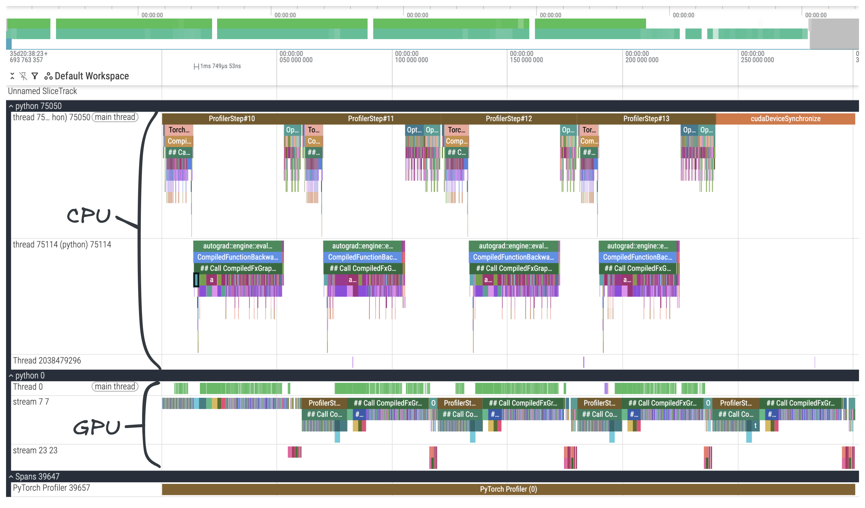
The upper tracks show CPU threads and operations on those threads, and the lower tracks show GPU streams and operations queued onto those streams. The CPU can launch multiple kernels to queue work on the GPU without waiting for previous kernels to complete.

From our code, we know that we've profiled four training steps and we can see that represented in the profiler trace. Let's focus in on one of the training steps so that we can see the different stages of it. We'll look at the CPU first, since that's where our program starts to run before launching kernels on the GPU.

CPU

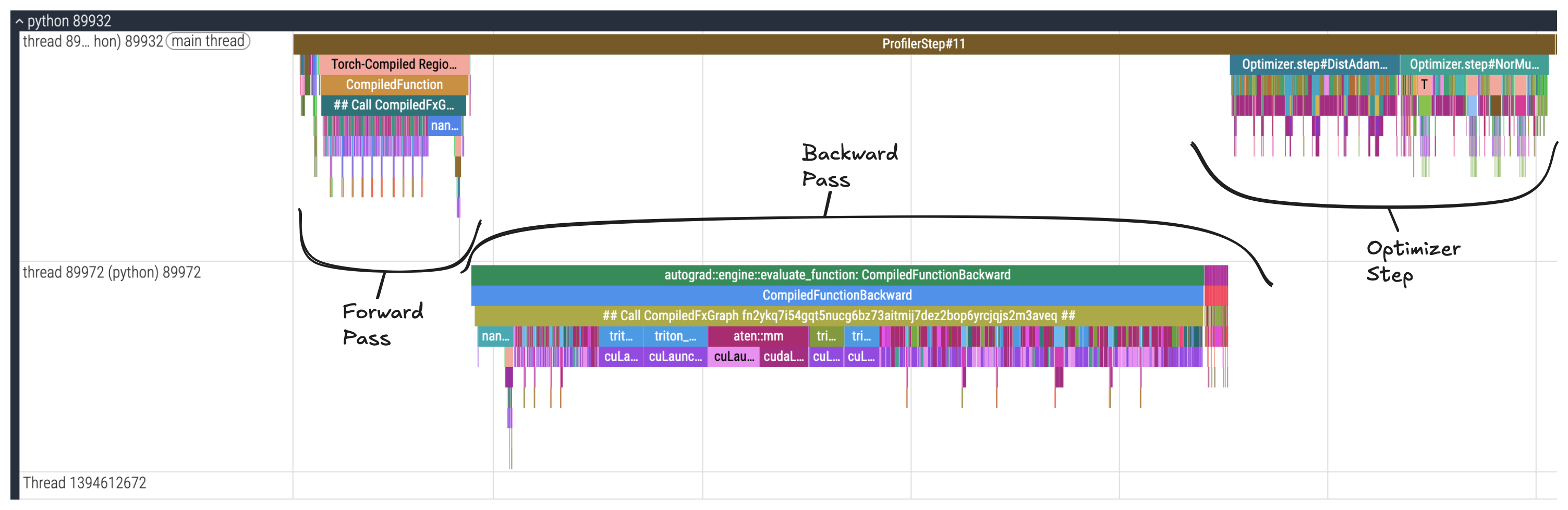
The image above is annotated to show the different phases of a training step. There's the forward and backward passes and the optimizer step where the gradients are used to update the weights.

We can zoom into each stage to look more closely. Each colored block is known as a "slice" and represents a single operation. The width of a slice corresponds to the operation's duration.

In the second image the flash_attn_3::fwd operation is selected, take note of the "Input Strides" and "Input Dims" sections. You'll notice they match the model_dim=768, num_heads=6, and head_dim=128 arguments passed in when we created our GPT model.

The fourth image shows the triton_poi_fused__unsafe_view_mul_sigmoid_view_6 operation includes some information about the GPU kernel it launches. Immediately below is the cuLaunchKernel slice representing the GPU kernel launch.

From CPU to GPU

We can hover over or click to select one of these slices and see that their category falls under cuda_runtime or cuda_driver, while other operations we saw were in the cpu_op category.

Now click on one of these slices you might notice something different; there's an orange line that extends out from it. Zooming out, we can see that that orange line is actually an arrow which points to a slice on the GPU track. The slice we've selected is launching a kernel on the GPU, and the slice that the arrow is pointing to represents the kernel operation on the GPU.

If we select the immediate next slice in the GPU track, we will see that there is a different arrow which points to that slice. Following the arrow to its origin brings us back to a cudaLaunchKernel, which was launched just after the memory copy kernel that we started from.

Now we can relate operations on the GPU stream to where they launched in the CPU. If we looked at the CPU thread for the backward pass, we would see CUDA kernels being launched there as well. Instead of manualy zooming in and out and following the arrow, we could also click the slice name in the "Following Flows" section.

Now, let's look at the GPU track in the profiler trace more closely.

GPU

Now that we've seen how CPU operations launch kernels, let's examine how those kernels execute on the GPU. When our code needs to use the GPU, it launches a kernel which gets enqueued onto a GPU stream where kernels are executed in FIFO order. Like we did for the CPU, let's look at one training step on the GPU.

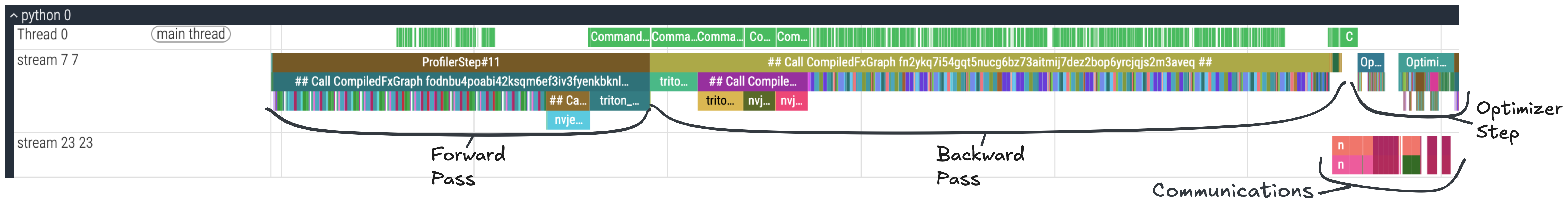
Same as before, we have our normal training step phases: the forward pass, backward pass, and the optimizer step at the end. Since the GPU stream operates as a queue, the GPU operations for all the stages of training execute in FIFO order.

You may notice that there are some gaps in the GPU stream. These gaps represent idle time when the GPU is not doing any computation. Ideally our profiler trace would show minimal gaps, with the GPU continuously executing kernels. Each gap is an opportunity for potential optimization.

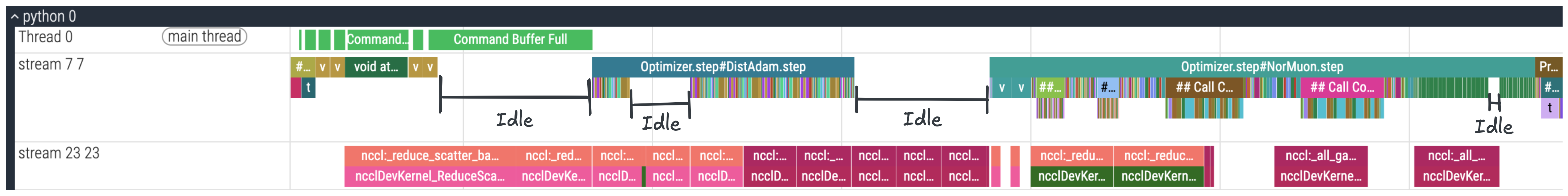
Just below the main GPU stream there are a few other slices on a separate stream. Modded-NanoGPT uses asynchronous communication operations which run on this separate GPU stream. In some places we can see that the communication slices overlap with computation slices in the main GPU stream above. Communications have latency and this overlap improves performance by keeping the GPU busy with computations instead of waiting idly for communications to complete.

Trace With Stacks

In order to reduce clutter when viewing the trace, so far our traces did not contain the call stack information because we've passed the with_stack=False argument to the profiler. If we want to correlate these operations with the exact file names and line numbers in code we can change this to with_stack=True. This will show the file name and the line number in each slice showing where the operation was called in code.

You can use the trace explorer below to explore what the profiler trace looks like with stack information.

HolisticTraceAnalysis

There is more information about the GPUs that can be extracted and visualized from the profiled output files. To do that we need to use the tensorboard_trace_handler function instead of export_chrome_trace. We need to use a different callback function which is passed to the on_trace_ready argument. Here's how to do it:

def trace_handler(prof: torch.profiler.profile):
    tb_handler = torch.profiler.tensorboard_trace_handler(
        "/root/mngpt-tb-traces",
        worker_name=f"gpu-rank-0{rank}",
        use_gzip=True,
    )
    tb_handler(prof)

While it is possible to use Tensorboard to load the files and view this information, Tensorboard integration with the PyTorch profiler is technically deprecated. To use it simply run tensorboard --logdir=/root/mngpt-tb-traces

A good alternative is the HolisticTraceAnalysis library. HolisticTraceAnalysis allows us to parse the data into Pandas dataframes, visualize it in charts, and analyze it by rank. The types of analysis in the HolisticTraceAnalysis include:

1. Temporal Breakdown - Breaks down GPU time spent into "idle", "compute", or "non-compute" time categories.
2. Idle Time Breakdown - Categorizes idle GPU time into "host", "kernel", or "other" wait categories.
3. Kernel Breakdown - Can be used to view time, call count, and other information for the different kernel types used during training.
4. Communication Computation Overlap - The amount of time concurrently communicating and computing divided by the total amount of time spent communicating.

Some of these metrics are shown in the below charts for Modded-NanoGPT:

The files generated by tensorboard_trace_handler can also be used to visualize the profiler trace as we did previously using either chrome://tracing or the Perfetto UI.

For a full list you can check out the docs.